Solving 1st and 2nd Order Linear ODEs with Constant Coefficients

In this post, I will cover the following:

• First-Order Linear Differential Equations (ODEs)

• Second-Order Linear Differential Equations (ODEs)

First-Order Linear Differential Equations (ODEs)

---

First, we'll look at first-order linear differential equations with constant coefficients, covering the homogeneous case where the right-hand side is zero, followed by the non-homogeneous case with a trigonometric term on the right-hand side.

Step-by-Step Solution (Homogeneous)

---

Step 1. Separation of Variables

Move the terms involving $y$ to the left and terms involving $t$ to the right (assuming \(y \neq 0\)):

$$\frac{dy}{dt}+Py = 0 \longrightarrow \frac{dy}{dt} = -Py \longrightarrow \frac{dy}{y} = -Pdt$$

(Note: If \(y = 0\), it trivially satisfies the equation, which is known as the trivial solution.)

Step 2. Integration

Integrate both sides with respect to their variables, combining the constants of integration into a single constant $c$ on the right:

$$\int\frac{dy}{y} = \int-Pdt \longrightarrow \ln|y| = -Pt + c$$

Step 3. Exponentiation and Solving for $y$

Exponentiate both sides with base $e$ to eliminate the natural logarithm:

$$e^{\ln|y|} = e^{-Pt+c} \longrightarrow |y| = e^ce^{-Pt}$$

Removing the absolute value gives:

$$y = \pm e^c e^{-Pt}$$

Since \(\pm e^c\) is simply an arbitrary non-zero constant, we can replace it with a single constant $C$. Allowing \(C = 0\) accounts for the trivial solution \(y = 0\), giving the general solution:

$$y = C e^{-Pt}$$

Step-by-Step Solution (Non-homogeneous)

---

Step 1. Problem Setup and Euler's Formula

$$\frac{dy}{dt} + Py = \cos(\omega t)$$

Before diving into the solution, recall Euler's formula, which connects complex exponentials with trigonometric functions:

$$e^{i\omega t} = \cos(\omega t) + i\sin(\omega t)$$

From this relation, cosine and sine can be represented as exponential forms:

$$\cos(\omega t) = \frac{e^{i\omega t} + e^{-i\omega t}}{2} \qquad \sin(\omega t) = \frac{e^{i\omega t} - e^{-i\omega t}}{2i}$$

Step 2. Trigonometric Synthesis Setup

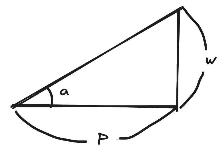
From this geometric relationship, the trigonometric components and the phase shift \(\alpha\) are defined as:

$$\cos\alpha = \frac{P}{\sqrt{P^2 + \omega^2}} \qquad \sin\alpha = \frac{\omega}{\sqrt{P^2 + \omega^2}} \qquad \alpha = \arctan\left(\frac{\omega}{P}\right)$$

Step 3: Variation of Parameters

we replace the constant $C$ with an unknown time-dependent function $C(t)$

$$y(t) = C(t) e^{-Pt}$$

Using the product rule, the first derivative of $y(t)$ is:

$$\frac{dy}{dt} = \frac{dC}{dt} e^{-Pt} - P C(t) e^{-Pt}$$

Substitute into the differential equation:

$$\left( \frac{dC}{dt} e^{-Pt} - P C(t) e^{-Pt} \right) + P \Big( C(t) e^{-Pt} \Big) = \cos(\omega t)$$

The terms involving \(PC(t)e^{-Pt}\) cancel each other out:

$$\frac{dC}{dt} e^{-Pt} = \cos(\omega t) \longrightarrow \frac{dC}{dt} = e^{Pt}\cos(\omega t)$$

Step 4. Solving for $C(t)$

Integrating both sides with respect to $t$ yields:

$$C(t) = \int e^{Pt}\cos(\omega t),dt = \frac{e^{Pt}}{\sqrt{P^2 + \omega^2}}\cos(\omega t - \alpha) + C_1$$

(Here, the harmonic addition formula was applied with phase angle α)

Finally, substituting $C(t)$ back into \(y(t) = C(t)e^{-Pt}\):

$$y(t) = \left( \frac{e^{Pt}}{\sqrt{P^2 + \omega^2}}\cos(\omega t - \alpha) + C_1 \right) e^{-Pt} = \frac{1}{\sqrt{P^2 + \omega^2}}\cos(\omega t - \alpha) + C_1 e^{-Pt}$$

Second-Order Linear Differential Equations (ODEs)

---

Next, we will cover second-order linear differential equations with constant coefficients, focusing on solving the homogeneous case.

$$\frac{d^2 y}{dt^2} + P_1 \frac{dy}{dt} + P_0 y = 0$$

Step-by-Step Solution (homogeneous)

---

Step 1. Form the Characteristic Equation

Assume a trial solution of exponential form:

$$y = e^{at}$$

Differentiating yields \(\frac{dy}{dt} = ae^{at}\) and \(\frac{d^2y}{dt^2} = a^2e^{at}\). Substituting these into the differential equation gives:

$$a^2 e^{at} + P_1 a e^{at} + P_0 e^{at} = 0$$

Dividing through by \(e^{at} \neq 0\), we obtain the characteristic equation:

$$a^2 + P_1 a + P_0 = 0$$

Step 2. Solve for the Roots

Using the quadratic formula, solve for the roots \(a_1\), \(a_2\):

$$a = \frac{-P_1 \pm \sqrt{P_1^2 - 4P_0}}{2}$$

Step 3. Determine the General Solution

Please note that in this post, we will not cover the case where \(P_1^2 - 4P_0 < 0\)(complex conjugate roots).

• Case 1: Two Distinct Real Roots (\(P_1^2 - 4P_0 > 0\))

  • General Solution:

$$y = C_1 e^{a_1t} + C_2 e^{a_2t}$$

• Case 2: Repeated Real Root (\(P_1^2 - 4P_0 = 0\))

  • Since a repeated root yields only \(e^{at}\), we apply the reduction of order method to find the second linearly independent solution, which results in \(te^{at}\).

  • General Solution:

$$y = C_1e^{at} + C_2 te^{at}$$

Now, by substituting the general solution \(y = C_1Y + C_2Z\) back into the original differential equation, we can see that it satisfies the equation as follows:

$$\frac{d^2}{dt^2}(C_1 Y + C_2 Z) + P_1 \frac{d}{dt}(C_1 Y + C_2 Z) + P_0 (C_1 Y + C_2 Z)$$

$$= C_1 \underbrace{\left(\frac{d^2 Y}{dt^2} + P_1 \frac{dY}{dt} + P_0 Y\right)}{= 0} + C_2 \underbrace{\left(\frac{d^2 Z}{dt^2} + P_1 \frac{dZ}{dt} + P_0 Z\right)}{= 0} = 0$$