Step-by-Step Quarter-Car Model Simulation in MATLAB

In this post, we will model a 2-DOF quarter-car system composed of a tire stiffness spring, an unsprung mass, and a sprung mass supported by a suspension spring and damper.

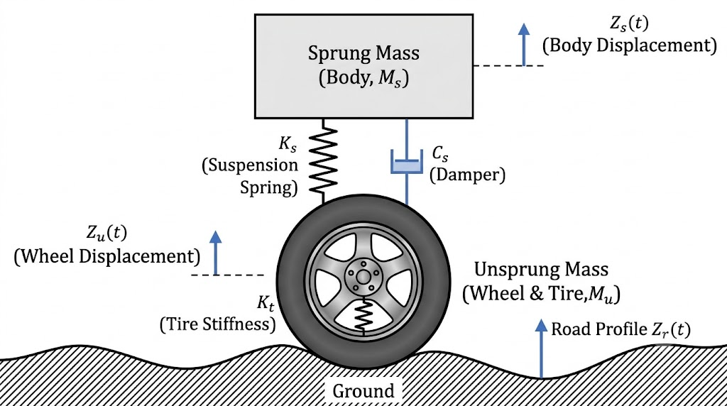
First, let's analyze the forces acting on the unsprung mass. Positioned between the tire spring below and the suspension (spring and damper) above, it is subject to interaction forces from both directions.

For example, when the road profile rises and compresses the tire, the tire spring pushes the wheel upward. Conversely, if the wheel moves upward relative to the vehicle body, the suspension between them is compressed, causing the suspension spring and damper to exert a downward reaction force on the wheel.

Unsprung Mass

Based on Newton's second law (\(F = ma\)), we sum the forces acting directly on \(m_u\):

• Force from the tire (\(F_t\)):

  Assuming the tire behaves as a linear spring, the compression of the tire is (\(z_r - z_u\)). When the road rises (\(z_r > z_u\)), it pushes the wheel upward:

  $$F_t = k_t (z_r - z_u)$$

• Force from the suspension (\(F_s\)):

  The suspension sits between the wheel (\(z_u\)) and the vehicle body (\(z_s\)). The relative compression is (\(z_u - z_s\)), and the relative compression velocity is (\(\dot{z}_u - \dot{z}_s\)). When the suspension is compressed, it resists by pushing the wheel downward (negative direction):

  $$F_s = -k_s (z_u - z_s) - c_s (\dot{z}_u - \dot{z}_s)$$

Combining both forces yields the net force acting on the unsprung mass:

$$F_{mu} = m_u \ddot{z}_u = F_t + F_s$$

Substituting the force expressions gives:

$$m_u \ddot{z}_u = k_t (z_r - z_u) - k_s (z_u - z_s) - c_s (\dot{z}_u - \dot{z}_s)$$

Rearranging all dependent state variables to the left-hand side and keeping the disturbance input (\(z_r\)) on the right-hand side gives the standard form:

$$m_u \ddot{z}_u + c_s (\dot{z}_u - \dot{z}_s) + (k_s + k_t) z_u - k_s z_s = k_t z_r$$

Next, we establish the governing equation for the vehicle body, represented by the sprung mass.

Unlike the unsprung mass, the sprung mass does not interact directly with the road; it is influenced solely by the suspension assembly connecting it to the wheel.

Sprung Mass

In the previous section, we defined the force exerted by the suspension on the unsprung mass as \(F_s\). According to Newton's third law, the force exerted on the sprung mass is equal in magnitude and opposite in direction. Applying Newton's second law directly to the sprung mass yields:

$$F_{ms} = m_s \ddot{z}_s = -F_s = k_s (z_u - z_s) + c_s (\dot{z}_u - \dot{z}_s)$$

Rearranging all state terms to the left-hand side yields the familiar standard form:

$$m_s \ddot{z}_s + c_s (\dot{z}_s - \dot{z}_u) + k_s (z_s - z_u) = 0$$

While the coupled second-order differential equations accurately describe the physical system, directly implementing them using individual integration blocks can result in cluttered wiring inside Simulink.

A far cleaner approach—and the foundation of modern control theory—is converting the system into State-Space representation:

$$\begin{aligned} \dot{x} &= Ax + Bu \\ y &= Cx + Du \end{aligned}$$

Where:

• \(x \in \mathbb{R}^{4 \times 1}\) is the state vector.

• \(u \in \mathbb{R}^{1 \times 1}\) is the input (road disturbance \(z_r\)).

• \(y \in \mathbb{R}^{p \times 1}\) is the output vector of interest.

• $A, B, C, D$ are system, input, output, and feedforward matrices, respectively.

Since this is a 2-DOF system governed by two second-order ODEs, we need four state variables representing the position and velocity of each mass:

$$x = \begin{bmatrix} x_1 \\ x_2 \\ x_3 \\ x_4 \end{bmatrix} = \begin{bmatrix} z_s \\ \dot{z}_s \\ z_u \\ \dot{z}_u \end{bmatrix}$$

• \(x_1 = z_s\): Sprung mass displacement

• \(x_2 = \dot{z}_s\): Sprung mass velocity

• \(x_3 = z_u\): Unsprung mass displacement

• \(x_4 = \dot{z}_u\): Unsprung mass velocity

System Matrices (\(\dot{x} = Ax + Bu\))

Arranging the equations of motion in terms of the state vector yields the system matrix A and input matrix B:

$$\begin{bmatrix} \dot{z}_s \\ \ddot{z}_s \\ \dot{z}_u \\ \ddot{z}_u \end{bmatrix} = \begin{bmatrix} 0 & 1 & 0 & 0 \\ -\frac{k_s}{m_s} & -\frac{c_s}{m_s} & \frac{k_s}{m_s} & \frac{c_s}{m_s} \\ 0 & 0 & 0 & 1 \\ \frac{k_s}{m_u} & \frac{c_s}{m_u} & -\frac{k_s + k_t}{m_u} & -\frac{c_s}{m_u} \end{bmatrix} \begin{bmatrix} z_s \\ \dot{z}_s \\ z_u \\ \dot{z}_u \end{bmatrix} + \begin{bmatrix} 0 \\ 0 \\ 0 \\ \frac{k_t}{m_u} \end{bmatrix} z_r$$

Output Equation (\(y = Cx + Du\))

To observe both the body displacement and wheel displacement as outputs:

$$y = \begin{bmatrix} z_s \\ z_u \end{bmatrix} = \begin{bmatrix} 1 & 0 & 0 & 0 \\ 0 & 0 & 1 & 0 \end{bmatrix} x + \begin{bmatrix} 0 \\ 0 \end{bmatrix} u$$

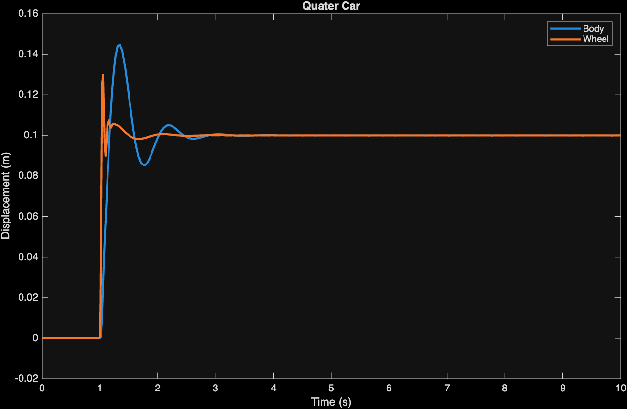
Running the simulation in MATLAB using the derived equations yields the following result:

The complete source code is provided below.

https://gist.github.com/RustSynx/7d5e6b324f022f42ccb118d68877e800