Demystifying OLS: The Engine Behind Linear Regression

When diving into linear regression, the very first engine you encounter is OLS (Ordinary Least Squares). In this post, we’ll explore the fundamental definition and mechanics of OLS, look into why it’s so powerful, examine where it critically falls short, and cover practical ways to address those limitations in real-world scenarios.

The Fundamental Definition and Mechanics of OLS

Linear regression models solved via OLS generally fall into two categories: Simple Linear Regression with a single explanatory variable (\(y = \beta_0 + \beta_1 x\)), and Multiple Linear Regression with two or more variables (\(y = \beta_0 + \beta_1 x_1 + \dots + \beta_k x_k\)). The crucial condition here is that the equation must be linear with respect to the parameters (\(\beta\)), regardless of the shape of the features (\(x\\\)).

How does OLS actually calculate these parameters? As the name suggests, it minimises the sum of squared errors through the most standard approach. Specifically, it finds the optimal coefficients by minimising the Sum of Squared Residuals (RSS)—the squared differences between the actual values (\(y\\\)) and the predicted values (\(\hat{y}\)):

$$\sum (y - \hat{y})^2$$

Ultimately, we substitute the prediction model (\(\hat{y} = \beta_0 + \beta_1 x\), or \(\hat{y} = \beta_0 + \beta_1 x_1 + \dots + \beta_k x_k\) for multiple variables) into the squared error formula. By taking the partial derivative with respect to each parameter (\(\beta\)) and setting it to zero, we derive a closed-form solution that calculates the optimal coefficients directly from the given \(x\\\) and \(y\\\) data in a single step.

Strengths and Limitations

Strengths

The first major strength of OLS is its computational efficiency. Instead of relying on iterative optimisation algorithms, it derives a unique closed-form solution through direct matrix operations. (With the caveat that the number of features remains within a reasonable scale—a limitation we will examine later.)

From an engineering perspective, it delivers reliable baseline performance at minimal computational cost. Furthermore, its clear mathematical foundation, theoretical rigour (such as the Gauss-Markov theorem), and high interpretability—where every coefficient (\(\beta\)) has a distinct and explainable meaning—solidify OLS as a timeless, reliable 'white-box' model.

Limitations

However, OLS comes with clear limitations and trade-offs.

1. Computational Bottleneck in High Dimensions (\(O(p^3)\))

As the number of features (\(p\\\)) grows, the cost of matrix inversion scales cubically. You might wonder: "Didn't we just say OLS is computationally fast?" In standard tabular business data—where features typically range from dozens to a few hundred—modern hardware solves it in milliseconds. However, in high-dimensional domains like genomics or NLP where features reach tens of thousands, exact matrix inversion becomes computationally prohibitive.

2. Undetermined Systems (\(n < p\\\))

A related and fatal issue occurs when the number of observations (\(n\\\)) is smaller than the number of features (\(p\\\)). Just like solving a system of equations with more variables than equations, there are infinite possible solutions. Mathematically, the matrix becomes non-invertible, making it impossible for OLS to find a unique set of parameters.

3. Restricted to Linearity in Parameters (\(\beta\))

As established in the definition, OLS is strictly bound to models linear in their parameters. It cannot inherently capture intricate, non-linear patterns without manual feature engineering.

4. The Achilles' Heel: Extreme Sensitivity to Outliers

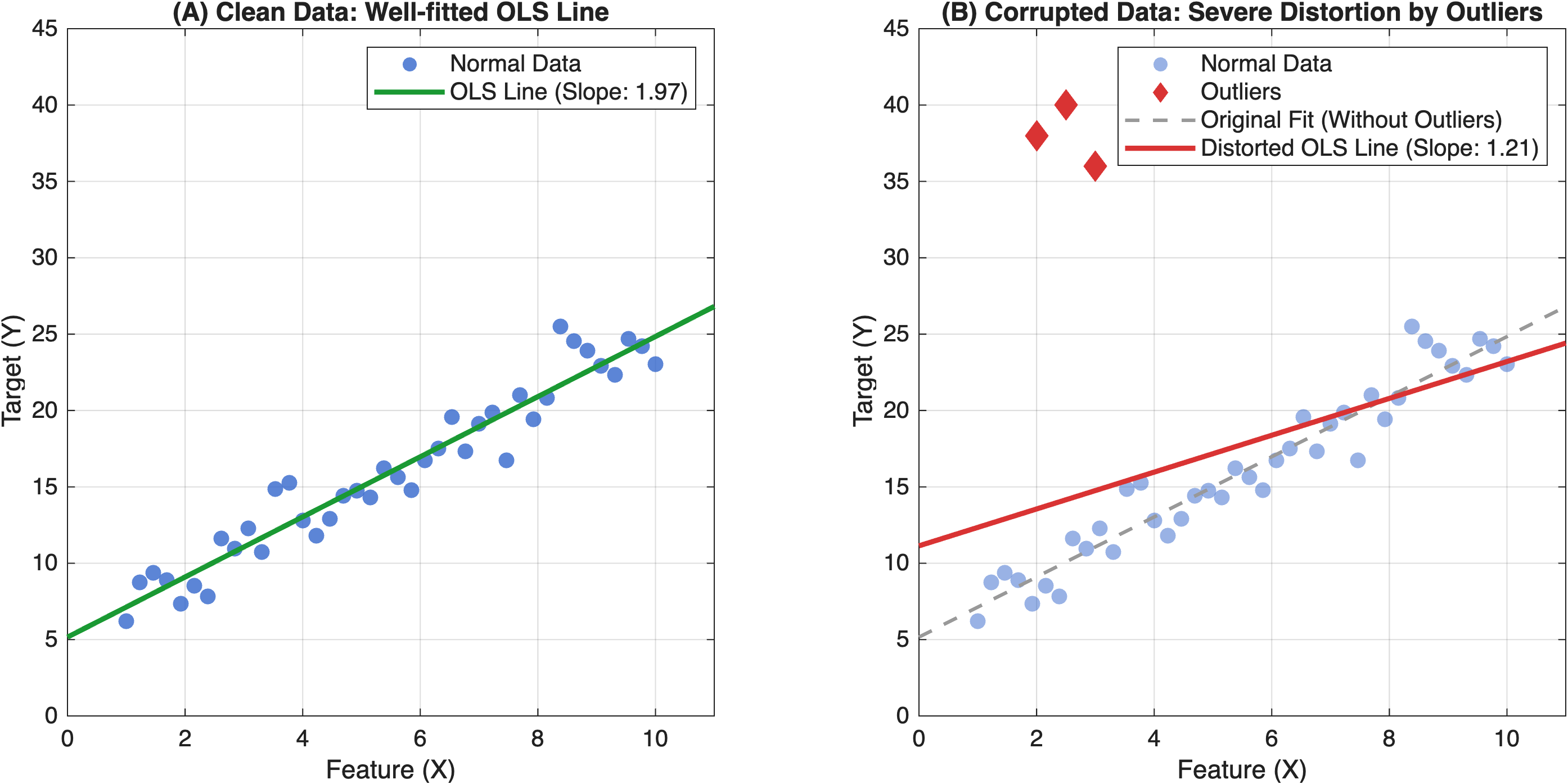
Perhaps the most critical flaw is its vulnerability to outliers. Because OLS minimizes squared errors, an outlier with a large deviation incurs an exponentially amplified penalty. To appease that single quadratic spike, the model will drag the entire regression line toward the outlier, sacrificing accuracy across the rest of the legitimate data.

Beyond Vanilla OLS: Ridge and Lasso

Among the best remedies for these limitations are Ridge (\(L_2\) regularisation) and Lasso (\(L_1\) regularisation).

By introducing penalty terms on the coefficients, these methods allow models to calculate unique solutions even when the number of features exceeds the number of observations (\(p \gt n\\\)), while mitigating overfitting and resolving multicollinearity.

For instance, when predicting housing prices using both 'square footage' and 'number of bedrooms', the strong linear correlation between these two features makes it hard for vanilla OLS to isolate their individual effects. Ridge and Lasso stabilise or select these coefficients, turning unstable estimations into reliable, generalisable models.

Ridge

$$\sum (y - \hat{y})^2 + \lambda \sum_{j=1}^p \beta_j^2$$

Here, \(\beta_j\) represents each slope coefficient. Because the penalty uses squared terms (\(L_2\)), the derivative still contains \(\beta_j\). Consequently, the shrinking force is proportional to the coefficient's magnitude—as \(\beta_j\) approaches zero, the penalty force weakens, shrinking coefficients close to zero without ever zeroing them out entirely.

Lasso

$$\sum (y - \hat{y})^2 + \lambda \sum_{j=1}^p \vert{}\beta_j\vert{}$$

Lasso adds the sum of absolute values (\(L_1\)) as a penalty. When differentiated (for \(\beta \neq 0\)), the variable \(\beta_j\) disappears completely, leaving only a constant sign (\(\pm 1\)). Because it applies a constant downward pressure regardless of the coefficient's size, weaker coefficients are subtracted all the way to exactly zero (Sparsity), effectively performing automatic feature selection.

Conclusion

OLS is far from an obsolete algorithm. Its computational speed, mathematical clarity, and unrivalled interpretability make it an enduring, essential baseline in any data practitioner’s toolkit.

When real-world complexities—such as multicollinearity, high dimensionality (\(p > n\\\)), or overfitting—threaten vanilla OLS, you don't always need to abandon linear models entirely. By understanding how Ridge stabilises correlated features and Lasso performs automatic feature selection, you can build linear models that are not only interpretable, but also robust and generalisable.